Getting started with kernel profiling
This notebook shows how to get started with kernel profiling.
Kernel profiling is the process of collecting detailed performance metrics to understand how kernels utilize GPU hardware and how closely they approach peak performance.
It helps identify performance bottlenecks and assess the impact of optimizations.
NVIDIA provides Nsight Compute for this purpose.
ReProspect enables a fully programmatic use of this tool: it launches it, reads the collected performance metrics into Python data structures, and supports analyses of these data that can go all the way to test assertions.
As an example, we consider a kernel that fills a buffer. In the reference case, each thread writes a single element. We programmatically analyze how restructuring the kernel so that each thread writes a batch of several elements, the static batch size, a compile-time parameter of the kernel, can improve performance.
About this page
This page is rendered from a Jupyter notebook, executed at documentation build time, located at docs/source/getting-started/example_kernel_profiling.ipynb in the repository.
To run the example yourself, download the notebook and open it in JupyterLab.
Alternatively, copy-paste the code snippets successively into an interactive Python session.
The requirements are Python 3.10 or newer and ReProspect.
The example also requires:
a CUDA Toolkit installation providing
nvcc;an Nsight Compute installation providing the command-line tool
ncu;the NVTX header
nvtx3/nvtx3.hpp(included in recent CUDA Toolkits; otherwise available from NVTX installation);a C++20-capable toolchain.
At the end, a final section “Going further” additionally uses the binary-analysis component and requires that the CUDA Toolkit installation provide cuobjdump and cu++filt.
That final section is optional and not needed for the rest of the notebook.
Because kernel profiling executes the program, a GPU is required.
In addition, kernel profiling requires sufficiently elevated access privileges (e.g., --cap-add=SYS_ADMIN for a Docker container; see also NVIDIA’s documentation).
Source code
We consider a kernel that writes a given value to each element of a buffer.
The kernel is parameterized by the compile-time parameter StaticBatchSize.
In the reference case, which corresponds to a static batch size equal to 1, each thread writes a single element:
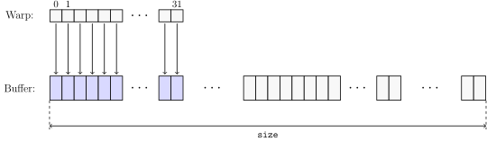
Reference kernel (StaticBatchSize equal to 1).
For values of the static batch size larger than 1, the kernel is restructured so that each thread performs StaticBatchSize writes to elements separated by work_stride, the total number of threads launched, as illustrated here for the case of a static batch size of 2:
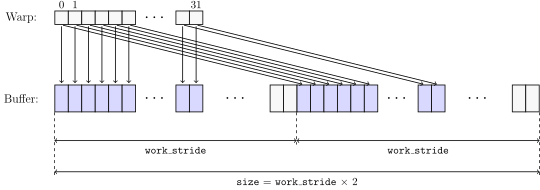
Restructured kernel (StaticBatchSize equal to 2).
The program launches the kernel to fill a buffer of 512 Mi elements (\(1024 \times 1024 \times 512\)), for elements of type char and of type int, corresponding to buffers of 0.5 GiB and 2 GiB, respectively, and for static batch sizes of 1, 2, 4, 8, 16 and 32.
The source code features NVTX annotations, for two purposes.
On the one hand, the outer NVTX range start_end_range delimits the kernel launches that Nsight Compute profiles: only launches within this range are collected.
In particular, the warm-up launches fall outside start_end_range and are not profiled.
On the other hand, the inner ranges provide convenient accessor paths for the collected data.
In particular, with the inner ranges char_range and int_range, each in turn with nested ranges static_batch_size_1, …, static_batch_size_32, each kernel launch falls within a specific nested range.
Below, we will look up the collected performance metrics by these ranges.
The ranges belong to a dedicated NVTX domain, which keeps them separate from other NVTX annotations, such as annotations that libraries used by an application may emit themselves.
The program also times each kernel execution and computes the corresponding throughput (GB/s).
Upon passing the option --print-throughputs, it prints these throughputs.
CODE = """
#include <array>
#include <cassert>
#include <chrono>
#include <format>
#include <iostream>
#include <source_location>
#include <sstream>
#include <stdexcept>
#include <string>
#include <string_view>
#include <utility>

#include <cuda_runtime.h>
#include <nvtx3/nvtx3.hpp>

inline void check_cudart_call(
    const cudaError_t status,
    const char* const statement,
    const std::source_location& loc = std::source_location::current()) {
    if (status != cudaSuccess) {
        std::ostringstream oss;
        oss << statement << " failed: " << status << " (" << cudaGetErrorName(status)
            << "): " << cudaGetErrorString(status) << " (" << loc.file_name() << ":" << loc.line() << ")";

        throw std::runtime_error(oss.str());
    }
}

#define CHECK_CUDART_CALL(statement) check_cudart_call((statement), #statement)

struct ExampleKernelProfilingDomain {
    static constexpr char const * name{"example_kernel_profiling_domain"};
};

template <unsigned int StaticBatchSize, typename T>
__global__ void fill_kernel(T* data, const T val, const unsigned int size) {
    const auto work_stride = blockDim.x * gridDim.x;
    const auto batch_stride = work_stride * StaticBatchSize;

    const unsigned int iwork = threadIdx.x + blockDim.x * blockIdx.x;
    for (unsigned int i = 0; i < batch_stride && i < size - iwork; i += work_stride) {
        data[iwork + i] = val;
    }
}

template <unsigned int StaticBatchSize, typename T>
void run_fill(cudaStream_t stream, T* data, const T val, const unsigned int size) {
    const std::string name = std::format("static_batch_size_{}", StaticBatchSize);
    const nvtx3::scoped_range_in<ExampleKernelProfilingDomain> range(name);

    constexpr unsigned int block_size = 128;

    assert(size % StaticBatchSize == 0);
    const unsigned int nwork = size / StaticBatchSize;

    const dim3 block(block_size, 1, 1);
    const dim3 grid((nwork + block_size - 1) / block_size, 1, 1);

    fill_kernel<StaticBatchSize><<<grid, block, 0, stream>>>(data, val, size);
    CHECK_CUDART_CALL(cudaStreamSynchronize(stream));
}

template <typename T, unsigned int... StaticBatchSizes>
auto timed_sweep(std::integer_sequence<unsigned int, StaticBatchSizes...>,
                 cudaStream_t stream, std::string_view label, const T val, const unsigned int size) {
    const std::string name = std::format("{}_range", label);
    const nvtx3::scoped_range_in<ExampleKernelProfilingDomain> range(name);

    T* data;
    CHECK_CUDART_CALL(cudaMallocAsync(&data, size * sizeof(T), stream));
    CHECK_CUDART_CALL(cudaStreamSynchronize(stream));

    const auto timed = [](auto&& f) {
        const auto start = std::chrono::high_resolution_clock::now();
        f();
        const auto end = std::chrono::high_resolution_clock::now();
        return end - start;
    };

    std::array<std::chrono::duration<double>, sizeof...(StaticBatchSizes)> timings{
        timed([&] { run_fill<StaticBatchSizes, T>(stream, data, val, size); })...
    };

    CHECK_CUDART_CALL(cudaFreeAsync(data, stream));
    CHECK_CUDART_CALL(cudaStreamSynchronize(stream));

    return timings;
}

int main(int argc, char* argv[]) {
    using StaticBatchSizeSequence = std::integer_sequence<unsigned int, 1, 2, 4, 8, 16, 32>;

    constexpr unsigned int size = 1024 * 1024 * 512;

    cudaStream_t stream;
    CHECK_CUDART_CALL(cudaStreamCreate(&stream));

    // Warmup. Avoid measuring module loading and other overhead.
    timed_sweep<char>(StaticBatchSizeSequence{}, stream, "char", 1, size);
    timed_sweep<int >(StaticBatchSizeSequence{}, stream, "int",  1, size);

    const auto start_end_range = nvtx3::start_range_in<ExampleKernelProfilingDomain>("start_end_range");

    const auto timings_char = timed_sweep<char>(StaticBatchSizeSequence{}, stream, "char", 1, size);
    const auto timings_int  = timed_sweep<int >(StaticBatchSizeSequence{}, stream, "int",  1, size);

    nvtx3::end_range_in<ExampleKernelProfilingDomain>(start_end_range);

    if (argc == 2 && std::string(argv[1]) == "--print-throughputs") {
        // Header.
        std::cout << std::format("{:<24}", "Static batch size");
        [&]<unsigned int... StaticBatchSizes>(std::integer_sequence<unsigned int, StaticBatchSizes...>) {
             ((std::cout << std::format(" | {:>7}", StaticBatchSizes)), ...);
        }(StaticBatchSizeSequence{});
        std::cout << std::endl;

        // Row char.
        std::cout << std::format("{:<24}", "Throughput - char (GB/s)");
        for (const auto& timing : timings_char) {
            std::cout << std::format(" | {:>7.1f}", sizeof(char) * size / (timing.count() * 1e9));
        }
        std::cout << std::endl;

        // Row int.
        std::cout << std::format("{:<24}", "Throughput - int (GB/s)");
        for (const auto& timing : timings_int) {
            std::cout << std::format(" | {:>7.1f}", sizeof(int) * size / (timing.count() * 1e9));
        }
        std::cout << std::endl;
    }

    CHECK_CUDART_CALL(cudaStreamDestroy(stream));
}
"""
Compilation
Because this example will execute the program, we compile the source code for the native architecture, i.e., the architecture of the GPU present on the machine.
import pathlib
import subprocess

from reprospect.utils import rich_helpers
from reprospect.utils.detect import GPUDetector

print(subprocess.check_output(('nvcc', '--version')).decode().strip())

print(subprocess.check_output(('ncu', '--version')).decode().strip())

visible_gpus = GPUDetector().detect()
print(f'Visible GPUs:\n{rich_helpers.to_string(rich_helpers.df_to_table(visible_gpus))}')

workdir = pathlib.Path.cwd() / 'example_kernel_profiling'
workdir.mkdir(exist_ok=True)
print(f'Working directory: {workdir}')

source = workdir / 'static_batch_size.cu'
executable = workdir / 'static_batch_size'

source.write_text(CODE)
_ = subprocess.check_call(('nvcc', '-arch=native', '-std=c++20', '-O3', '-o', executable, source))
nvcc: NVIDIA (R) Cuda compiler driver
Copyright (c) 2005-2026 NVIDIA Corporation
Built on Mon_Aug_03_13:24:11_PDT_2026
Cuda compilation tools, release 13.4, V13.4.59
Build cuda_13.4.r13.4/compiler.38657139_0
NVIDIA (R) Nsight Compute Command Line Profiler
Copyright (c) 2018-2026 NVIDIA Corporation
Version 2026.3.0.0 (build 38525999) (public-release)
Visible GPUs:
┏━━━━━━━━━━━━━━━━━━━━━━━━━━━━━━━━━━━━━━━━━━┳━━━━━━━┳━━━━━━━━━━━━━━━━━━━━━━━━━━━━┳━━━━━━━━━━━━━┳━━━━━━━━━━━━━━┓
┃ uuid                                     ┃ index ┃ name                       ┃ compute_cap ┃ architecture ┃
┡━━━━━━━━━━━━━━━━━━━━━━━━━━━━━━━━━━━━━━━━━━╇━━━━━━━╇━━━━━━━━━━━━━━━━━━━━━━━━━━━━╇━━━━━━━━━━━━━╇━━━━━━━━━━━━━━┩
│ GPU-d27df728-7612-809e-697e-38da9785efa3 │ 0     │ NVIDIA GeForce RTX 5070 Ti │ 12.0        │ BLACKWELL120 │
│ GPU-f0b17181-5e70-f633-ed96-14cf7e77e8e9 │ 1     │ NVIDIA GeForce RTX 5070 Ti │ 12.0        │ BLACKWELL120 │
└──────────────────────────────────────────┴───────┴────────────────────────────┴─────────────┴──────────────┘

Working directory: /tmp/tmp21llwp1j/example_kernel_profiling
Measured throughputs
Let us run the program with the option --print-throughputs.
This is a bare, unprofiled run: execution times measured by the program itself while profiling are not meaningful because the profiler may replay kernels and lock clocks, as described here.
Our program performs a warmup phase that launches each kernel once before the timed sweep, so that one-time effects such as lazy module loading do not affect the time measurements.
_ = subprocess.check_call((executable, '--print-throughputs'))
Static batch size        |       1 |       2 |       4 |       8 |      16 |      32
Throughput - char (GB/s) |   266.9 |   541.4 |   857.7 |   832.0 |   829.6 |   841.4
Throughput - int (GB/s)  |   852.2 |   844.7 |   839.0 |   833.3 |   830.7 |   826.7
We can observe that for the type char, the reference kernel (with a static batch size of 1) achieves a throughput that is about three times lower than the highest throughputs measured across the scenarios.
The measured throughput increases with the batch size and plateaus from a batch size of 4.
For the type int, the reference kernel already achieves the plateau performance.
The plateau is common to both element types.
It is tempting to hypothesize that the batching improves the memory access pattern. However, as the figures above illustrate, the reference kernel is already such that consecutive lanes of a warp write to consecutive elements in the buffer, and the restructured kernels preserve this memory access pattern. Improved coalescing thus cannot explain the increased throughput.
The kernel profiling that follows will let us assert that the memory accesses are coalesced at every static batch size, and identify the mechanism that actually drives the performance improvement.
Kernel profiling metrics
Nsight Compute categorizes metrics into counter metrics, ratio metrics and throughput metrics.
Counter metrics have four sub-metrics under them: the so-called roll-ups .sum, .avg, .min and .max, which represent different ways of aggregating counts across all instances of the hardware unit that the metric is associated with.
For instance, the counter metric smsp__inst_executed.sum represents the sum of all warp-level instructions executed across all streaming multiprocessor sub-partitions (SMSPs).
Sub-metrics can in turn have further sub-metrics under them, holding derived quantities calculated by Nsight Compute.
For instance, Nsight Compute has a database with peak values that certain sub-metrics may reach, and it can thus calculate for such sub-metrics the percentage of the peak that the collected value attains (e.g. .pct_of_peak_sustained_elapsed).
Ratio metrics have the roll-ups .pct, .ratio and .max_rate instead.
Throughput metrics always require sub-metric paths with multiple components.
ReProspect represents such metrics as typed objects.
They provide the names that must be passed to Nsight Compute to request collection, as well as the labels under which ReProspect will store the collected values for analysis.
A counter metric is constructed from its Nsight Compute base name, an optional human-readable pretty name, and one or several typed sub-metric paths (reprospect.tools.ncu.metrics.MetricCounter).
The Nsight Compute names are assembled by joining the base name with each sub-metric path, and the labels are obtained by joining the pretty name with a pretty rendering of the sub-metric paths, omitting sub-metric path components that ReProspect considers default, namely, .sum for counter metrics and .ratio for ratio metrics.
from reprospect.tools.ncu import MetricCounter, MetricCounterRollUp

inst_executed = MetricCounter(name='smsp__inst_executed', pretty_name='Executed instructions', subs=(MetricCounterRollUp.SUM,))

inst_executed_labels, inst_executed_names = inst_executed.labels(), inst_executed.gather()
print(inst_executed_labels, inst_executed_names)
('Executed instructions',) ('smsp__inst_executed.sum',)
For commonly used metrics, ReProspect provides targeted factories that encapsulate the Nsight Compute names and human-readable pretty names, such as the class reprospect.tools.ncu.metrics.L1TEXCache for metrics for memory workload analysis.
The metrics for this example combine factory-provided and directly constructed metrics:
from reprospect.tools.ncu import (
    L1TEXCache,
    LaunchGrid,
    MetricCounterRollUpQuantity,
    WarpStall,
    gather,
    labels,
)

metrics = (
    # Launch grid sizes.
    *LaunchGrid.create(dims=('x',)),
    # Overall instruction count.
    inst_executed,
    # L1/TEX cache memory traffic.
    *L1TEXCache.GlobalStore.Instructions.create(),
    *L1TEXCache.GlobalStore.Requests.create(),
    *L1TEXCache.GlobalStore.Sectors.create(),
    # Warp stall reasons.
    *WarpStall.ShortScoreboard.create(),
    *WarpStall.LGThrottle.create(),
    *WarpStall.LongScoreboard.create(),
    # DRAM memory traffic.
    MetricCounter(name='dram__bytes_op_write', pretty_name='Device memory store utilization', subs=((MetricCounterRollUp.SUM, MetricCounterRollUpQuantity.PCT_OF_PEAK_SUSTAINED_ELAPSED),)),
)

metric_labels, metric_names = labels(metrics), gather(metrics)

print(f'Metrics:\n{rich_helpers.to_string(rich_helpers.rows_to_table(zip(metric_labels, metric_names, strict=True), columns=("Label", "Name")))}')
Metrics:
┏━━━━━━━━━━━━━━━━━━━━━━━━━━━━━━━━━━━━━━━━━━━━━━━━━━━━━┳━━━━━━━━━━━━━━━━━━━━━━━━━━━━━━━━━━━━━━━━━━━━━━━━━━━━━━━━━━━━━━━━━━━━━━━━━━━┓
┃ Label                                               ┃ Name                                                                      ┃
┡━━━━━━━━━━━━━━━━━━━━━━━━━━━━━━━━━━━━━━━━━━━━━━━━━━━━━╇━━━━━━━━━━━━━━━━━━━━━━━━━━━━━━━━━━━━━━━━━━━━━━━━━━━━━━━━━━━━━━━━━━━━━━━━━━━┩
│ Launch grid size x                                  │ launch__grid_dim_x                                                        │
│ Executed instructions                               │ smsp__inst_executed.sum                                                   │
│ L1/TEX cache global store sass instructions         │ smsp__sass_inst_executed_op_global_st.sum                                 │
│ L1/TEX cache global store requests                  │ l1tex__t_requests_pipe_lsu_mem_global_op_st.sum                           │
│ L1/TEX cache global store sectors                   │ l1tex__t_sectors_pipe_lsu_mem_global_op_st.sum                            │
│ Warp stall short scoreboard                         │ smsp__average_warps_issue_stalled_short_scoreboard_per_issue_active.ratio │
│ Warp stall LG throttle                              │ smsp__average_warps_issue_stalled_lg_throttle_per_issue_active.ratio      │
│ Warp stall long scoreboard                          │ smsp__average_warps_issue_stalled_long_scoreboard_per_issue_active.ratio  │
│ Device memory store utilization (% of peak elapsed) │ dram__bytes_op_write.sum.pct_of_peak_sustained_elapsed                    │
└─────────────────────────────────────────────────────┴───────────────────────────────────────────────────────────────────────────┘
The requested L1/TEX cache memory traffic metrics are counter metrics that provide respectively the number of store instructions the SMSPs execute to write to global memory, the number of requests these store instructions generate to the memory system, and the number of sectors, i.e., aligned contiguous 32-byte chunks of global memory, these requests access; see also Nsight Compute’s documentation on the hardware model, as well as this presentation.
The requested warp stall reason metrics are ratio metrics that provide the average number of cycles that warps spend in the associated stalled state per issued instruction.
Running kernel profiling
Nsight Compute provides the command-line tool ncu for collecting performance metrics.
Here, we invoke it through the ReProspect class reprospect.tools.ncu.session.Session.
The argument executable designates the executable on which to collect data.
The argument nvtx_includes specifies one or several NVTX ranges to delimit the kernel launches that ncu profiles.
The value 'example_kernel_profiling_domain@start_end_range' follows the ncu convention <domain>@<range>.
The argument output determines the output file; for the passed value workdir / executable.name, the report is written to workdir / f'{executable.name}.ncu-rep'.
from reprospect.tools.ncu import Command, Session

nc = Session(
    command=Command(
        executable=executable,
        output=workdir / executable.name,
        metrics=metrics,
        nvtx_includes=('example_kernel_profiling_domain@start_end_range',),
    ),
)

nc.run(cwd=workdir)
Kernel profiling results
Nsight Compute provides the Python module ncu_report for low-level access to the output file generated by ncu.
The ReProspect class reprospect.tools.ncu.report.Report relies on ncu_report and adds infrastructure around it.
Its method extract_results_in_range() retrieves the collected performance metrics.
from reprospect.tools.ncu import Report

report = Report(command=nc.command)

results = report.extract_results_in_range(metrics=metrics)
The method extract_results_in_range() returns a ProfilingResults hierarchical data structure, in which the collected performance metrics are organised by nested NVTX range.
Each leaf node holds the performance metrics collected for one kernel launch, as a mapping from metric label to value.
The profiling results can then be queried by their NVTX path:
results_char = results.query(accessors=('char_range',))

print(results_char)
Profiling results
├── static_batch_size_1
│   └── fill_kernel-0
│       ├── Launch grid size x: 4194304
│       ├── Executed instructions: 335544320.0
│       ├── L1/TEX cache global store sass instructions: 16777216.0
│       ├── L1/TEX cache global store requests: 16777216.0
│       ├── L1/TEX cache global store sectors: 16777216.0
│       ├── Warp stall short scoreboard: 2.231566753983498
│       ├── Warp stall LG throttle: 0.0
│       ├── Warp stall long scoreboard: 0.0
│       ├── Device memory store utilization (% of peak elapsed): 27.079383010451348
│       ├── mangled: _Z11fill_kernelILj1EcEvPT0_S0_j
│       └── demangled: void fill_kernel<(unsigned int)1, char>(T2 *, T2, unsigned int)
├── static_batch_size_2
│   └── fill_kernel-1
│       ├── Launch grid size x: 2097152
│       ├── Executed instructions: 293601280.0
│       ├── L1/TEX cache global store sass instructions: 16777216.0
│       ├── L1/TEX cache global store requests: 16777216.0
│       ├── L1/TEX cache global store sectors: 16777216.0
│       ├── Warp stall short scoreboard: 1.4524685314723425
│       ├── Warp stall LG throttle: 1.3623918805803571e-08
│       ├── Warp stall long scoreboard: 0.0029636893953595843
│       ├── Device memory store utilization (% of peak elapsed): 54.81492171660284
│       ├── mangled: _Z11fill_kernelILj2EcEvPT0_S0_j
│       └── demangled: void fill_kernel<(unsigned int)2, char>(T2 *, T2, unsigned int)
├── static_batch_size_4
│   └── fill_kernel-2
│       ├── Launch grid size x: 1048576
│       ├── Executed instructions: 205520896.0
│       ├── L1/TEX cache global store sass instructions: 16777216.0
│       ├── L1/TEX cache global store requests: 16777216.0
│       ├── L1/TEX cache global store sectors: 16777216.0
│       ├── Warp stall short scoreboard: 2.5010923074216262
│       ├── Warp stall LG throttle: 0.6861679553985596
│       ├── Warp stall long scoreboard: 2.8077830489800903
│       ├── Device memory store utilization (% of peak elapsed): 89.8266306437145
│       ├── mangled: _Z11fill_kernelILj4EcEvPT0_S0_j
│       └── demangled: void fill_kernel<(unsigned int)4, char>(T2 *, T2, unsigned int)
├── static_batch_size_8
│   └── fill_kernel-3
│       ├── Launch grid size x: 524288
│       ├── Executed instructions: 161480704.0
│       ├── L1/TEX cache global store sass instructions: 16777216.0
│       ├── L1/TEX cache global store requests: 16777216.0
│       ├── L1/TEX cache global store sectors: 16777216.0
│       ├── Warp stall short scoreboard: 2.259319039134236
│       ├── Warp stall LG throttle: 3.495034446964016
│       ├── Warp stall long scoreboard: 7.696726501762093
│       ├── Device memory store utilization (% of peak elapsed): 90.81601400919533
│       ├── mangled: _Z11fill_kernelILj8EcEvPT0_S0_j
│       └── demangled: void fill_kernel<(unsigned int)8, char>(T2 *, T2, unsigned int)
├── static_batch_size_16
│   └── fill_kernel-4
│       ├── Launch grid size x: 262144
│       ├── Executed instructions: 139460608.0
│       ├── L1/TEX cache global store sass instructions: 16777216.0
│       ├── L1/TEX cache global store requests: 16777216.0
│       ├── L1/TEX cache global store sectors: 16777216.0
│       ├── Warp stall short scoreboard: 1.3369858462111395
│       ├── Warp stall LG throttle: 5.7679502874388735
│       ├── Warp stall long scoreboard: 10.464752613153673
│       ├── Device memory store utilization (% of peak elapsed): 90.98016094234166
│       ├── mangled: _Z11fill_kernelILj16EcEvPT0_S0_j
│       └── demangled: void fill_kernel<(unsigned int)16, char>(T2 *, T2, unsigned int)
└── static_batch_size_32
    └── fill_kernel-5
        ├── Launch grid size x: 131072
        ├── Executed instructions: 128450560.0
        ├── L1/TEX cache global store sass instructions: 16777216.0
        ├── L1/TEX cache global store requests: 16777216.0
        ├── L1/TEX cache global store sectors: 16777216.0
        ├── Warp stall short scoreboard: 0.7256462564273757
        ├── Warp stall LG throttle: 12.5702610327273
        ├── Warp stall long scoreboard: 13.715232016115774
        ├── Device memory store utilization (% of peak elapsed): 87.50615411628611
        ├── mangled: _Z11fill_kernelILj32EcEvPT0_S0_j
        └── demangled: void fill_kernel<(unsigned int)32, char>(T2 *, T2, unsigned int)
Between an innermost NVTX range and the metrics for a kernel launch, the hierarchy contains one more intermediate level.
In the profiling results tree shown above, this last intermediate level corresponds to the keys fill_kernel-0, …, fill_kernel-5.
The keys concatenate the kernel name with the index of the corresponding ncu action representing the kernel launch in the .ncu-rep report.
This level exists because an NVTX range may in general contain several kernel launches.
In our example, each innermost NVTX range contains exactly one kernel launch.
Hence, the NVTX range path suffices to identify each kernel launch, and the key of the last intermediate level is not needed.
For such cases, the class ProfilingResults provides a convenience method query_single_next_metrics() that allows the collected profiling metrics for a kernel launch to be retrieved directly from the NVTX range path, without specifying the key of the last intermediate level.
key_char_2, metrics_char_2 = results.query_single_next_metrics(accessors=('char_range', 'static_batch_size_2'))

inst_executed_char_2 = metrics_char_2["Executed instructions"]

print(f'Instructions executed for kernel launch {key_char_2}: {inst_executed_char_2}')
Instructions executed for kernel launch fill_kernel-1: 293601280.0
Interpreting kernel profiling results
From the ProfilingResults tree, the collected profiling metrics can be readily read into other Python data structures for further post-processing.
Here, we gather the collected performance metrics into a pandas.DataFrame to help with interpreting the results.
import pandas as pd

BATCH_SIZES = (1, 2, 4, 8, 16, 32)

metrics_char = {
    batch_size: dict(results.query_single_next_metrics(('char_range', f'static_batch_size_{batch_size}'))[1])
    for batch_size in BATCH_SIZES
}

df_char = pd.DataFrame.from_dict(metrics_char, orient='index')

selected = [
    'Launch grid size x',
    'Executed instructions',
    'Warp stall LG throttle',
    'Device memory store utilization (% of peak elapsed)',
]

print(rich_helpers.to_string(rich_helpers.df_to_table(df_char[selected].T, show_index=True)))
┏━━━━━━━━━━━━━━━━━━━━━━━━━━━━━━━━━━━━━━━━━━━━━━━━━━━━━┳━━━━━━━━━━━━━━━━━━━━┳━━━━━━━━━━━━━━━━━━━━━━━━┳━━━━━━━━━━━━━━━━━━━━┳━━━━━━━━━━━━━━━━━━━┳━━━━━━━━━━━━━━━━━━━━┳━━━━━━━━━━━━━━━━━━━┓
┃                                                     ┃ 1                  ┃ 2                      ┃ 4                  ┃ 8                 ┃ 16                 ┃ 32                ┃
┡━━━━━━━━━━━━━━━━━━━━━━━━━━━━━━━━━━━━━━━━━━━━━━━━━━━━━╇━━━━━━━━━━━━━━━━━━━━╇━━━━━━━━━━━━━━━━━━━━━━━━╇━━━━━━━━━━━━━━━━━━━━╇━━━━━━━━━━━━━━━━━━━╇━━━━━━━━━━━━━━━━━━━━╇━━━━━━━━━━━━━━━━━━━┩
│ Launch grid size x                                  │ 4194304.0          │ 2097152.0              │ 1048576.0          │ 524288.0          │ 262144.0           │ 131072.0          │
│ Executed instructions                               │ 335544320.0        │ 293601280.0            │ 205520896.0        │ 161480704.0       │ 139460608.0        │ 128450560.0       │
│ Warp stall LG throttle                              │ 0.0                │ 1.3623918805803571e-08 │ 0.6861679553985596 │ 3.495034446964016 │ 5.7679502874388735 │ 12.5702610327273  │
│ Device memory store utilization (% of peak elapsed) │ 27.079383010451348 │ 54.81492171660284      │ 89.8266306437145   │ 90.81601400919533 │ 90.98016094234166  │ 87.50615411628611 │
└─────────────────────────────────────────────────────┴────────────────────┴────────────────────────┴────────────────────┴───────────────────┴────────────────────┴───────────────────┘
From this representation of the collected profiling metrics, we can readily observe that as the static batch size increases, the number of executed instructions decreases. Indeed, each warp must execute certain instructions only once, such as those that determine each thread’s position in the grid and load the kernel’s parameters. As the static batch size increases, this once-per-warp instruction count is amortized over the batch.
We can bring this observation more to the forefront by calculating the number of executed instructions on a per-lane and per-stored-element basis:
WARP_SIZE = 32
ELEMENT_COUNT = 1024 * 1024 * 512

print(rich_helpers.to_string(rich_helpers.ds_to_table(df_char['Executed instructions'] * WARP_SIZE / ELEMENT_COUNT)))
┏━━━━━━┳━━━━━━┳━━━━━━━┳━━━━━━━┳━━━━━━━━┳━━━━━━━━━┓
┃ 1    ┃ 2    ┃ 4     ┃ 8     ┃ 16     ┃ 32      ┃
┡━━━━━━╇━━━━━━╇━━━━━━━╇━━━━━━━╇━━━━━━━━╇━━━━━━━━━┩
│ 20.0 │ 17.5 │ 12.25 │ 9.625 │ 8.3125 │ 7.65625 │
└──────┴──────┴───────┴───────┴────────┴─────────┘
The number is highest for the reference kernel. As the static batch size increases, it decays toward the count needed for the kernel’s loop alone, i.e., the instructions that update the address, execute the store, evaluate the loop condition, and branch.
As a result of most of the executed instructions being once-per-warp instructions rather than stores, the reference kernel executes store instructions, and thus feeds the memory system with bytes to be stored, at a rate below the rate that the memory system can sustain. As the static batch size increases and the once-per-warp instruction count becomes relatively less significant, store instructions are issued more rapidly and the memory system becomes the limiting resource. This interpretation is also consistent with the increase of the LG throttle warp stall reason metric, which is associated with warps stalled on issuing a local or global memory instruction because the corresponding L1/TEX cache queue is full.
For the type int, each store instruction feeds four times the bytes to the memory system, which explains that the reference kernel already sits on the plateau.
metrics_int = {
    batch_size: dict(results.query_single_next_metrics(('int_range', f'static_batch_size_{batch_size}'))[1])
    for batch_size in BATCH_SIZES
}

df_int = pd.DataFrame.from_dict(metrics_int, orient='index')

print(rich_helpers.to_string(rich_helpers.df_to_table(df_int[selected].T, show_index=True)))
┏━━━━━━━━━━━━━━━━━━━━━━━━━━━━━━━━━━━━━━━━━━━━━━━━━━━━━┳━━━━━━━━━━━━━━━━━━━━━┳━━━━━━━━━━━━━━━━━━━━┳━━━━━━━━━━━━━━━━━━━┳━━━━━━━━━━━━━━━━━━━━┳━━━━━━━━━━━━━━━━━━━┳━━━━━━━━━━━━━━━━━━━┓
┃                                                     ┃ 1                   ┃ 2                  ┃ 4                 ┃ 8                  ┃ 16                ┃ 32                ┃
┡━━━━━━━━━━━━━━━━━━━━━━━━━━━━━━━━━━━━━━━━━━━━━━━━━━━━━╇━━━━━━━━━━━━━━━━━━━━━╇━━━━━━━━━━━━━━━━━━━━╇━━━━━━━━━━━━━━━━━━━╇━━━━━━━━━━━━━━━━━━━━╇━━━━━━━━━━━━━━━━━━━╇━━━━━━━━━━━━━━━━━━━┩
│ Launch grid size x                                  │ 4194304.0           │ 2097152.0          │ 1048576.0         │ 524288.0           │ 262144.0          │ 131072.0          │
│ Executed instructions                               │ 285212672.0         │ 260046848.0        │ 180355072.0       │ 140509184.0        │ 120586240.0       │ 110624768.0       │
│ Warp stall LG throttle                              │ 0.12636128243278055 │ 2.7357731596116097 │ 9.468355777651764 │ 14.694058076659244 │ 28.51357766856318 │ 73.68056743856854 │
│ Device memory store utilization (% of peak elapsed) │ 91.02533955005879   │ 91.37357956051179  │ 91.94526498387951 │ 91.21756050033797  │ 90.26748730159836 │ 89.7038810963684  │
└─────────────────────────────────────────────────────┴─────────────────────┴────────────────────┴───────────────────┴────────────────────┴───────────────────┴───────────────────┘
Assertions on kernel profiling results
With the collected data gathered in Python data structures, the analysis can go all the way to test assertions. Here, we encode the main findings of the analysis in test assertions and verify programmatically the performance of the restructured kernel.
First, we verify that the memory access pattern is coalesced at every batch size.
We thus assert that each warp-level global store instruction generates one warp-level global store request that accesses one 32-byte sector (32 lanes \(\times\) 1 byte) for type char and four 32-byte sectors (32 lanes \(\times\) 4 bytes) for type int.
SECTOR_SIZE = 32 # byte

for (metrics_type, size_of_type) in ((metrics_char, 1), (metrics_int, 4)):
    for batch_size in BATCH_SIZES:
        m = metrics_type[batch_size]
        assert m['L1/TEX cache global store requests'] == m['L1/TEX cache global store sass instructions']
        assert m['L1/TEX cache global store sectors'] / m['L1/TEX cache global store requests'] == WARP_SIZE * size_of_type / SECTOR_SIZE
Next, we verify that the number of executed instructions decreases with the static batch size.
import itertools

for metrics_type in (metrics_char, metrics_int):
    inst_executed_type = [metrics_type[batch_size]['Executed instructions'] for batch_size in BATCH_SIZES]
    assert all(a >= b for a, b in itertools.pairwise(inst_executed_type))

    # The reduction is significant.
    assert metrics_type[16]['Executed instructions'] < metrics_type[1]['Executed instructions'] / 2
Finally, we verify the performance. For the static batch sizes belonging to the throughput plateau observed in the unprofiled run, we verify that device-memory write utilization remains above 70% of the peak sustained rate. The margin of 70% is well below the observed ~85%, to absorb run-to-run noise.
MIN_DEVICE_MEMORY_WRITE_UTILIZATION_PCT = 70 # percent

for (metrics_type, plateau_batch_sizes_type) in ((metrics_char, (4, 8, 16, 32)), (metrics_int, (1, 2, 4, 8, 16, 32))):
    for batch_size in plateau_batch_sizes_type:
        assert metrics_type[batch_size]['Device memory store utilization (% of peak elapsed)'] >= MIN_DEVICE_MEMORY_WRITE_UTILIZATION_PCT
Going further: insight through binary analysis
Inspecting the compiled CUDA assembly (SASS) code can be helpful to interpret kernel profiling results.
ReProspect’s binary-analysis component can be readily used for this purpose.
Here, we will look at the SASS code to interpret the two warp stall reason metrics that remain to be explained: the short and long scoreboard stalls.
print(rich_helpers.to_string(rich_helpers.df_to_table(df_char[['Warp stall short scoreboard', 'Warp stall long scoreboard']].T, show_index=True)))
┏━━━━━━━━━━━━━━━━━━━━━━━━━━━━━┳━━━━━━━━━━━━━━━━━━━┳━━━━━━━━━━━━━━━━━━━━━━━┳━━━━━━━━━━━━━━━━━━━━┳━━━━━━━━━━━━━━━━━━━┳━━━━━━━━━━━━━━━━━━━━┳━━━━━━━━━━━━━━━━━━━━┓
┃                             ┃ 1                 ┃ 2                     ┃ 4                  ┃ 8                 ┃ 16                 ┃ 32                 ┃
┡━━━━━━━━━━━━━━━━━━━━━━━━━━━━━╇━━━━━━━━━━━━━━━━━━━╇━━━━━━━━━━━━━━━━━━━━━━━╇━━━━━━━━━━━━━━━━━━━━╇━━━━━━━━━━━━━━━━━━━╇━━━━━━━━━━━━━━━━━━━━╇━━━━━━━━━━━━━━━━━━━━┩
│ Warp stall short scoreboard │ 2.231566753983498 │ 1.4524685314723425    │ 2.5010923074216262 │ 2.259319039134236 │ 1.3369858462111395 │ 0.7256462564273757 │
│ Warp stall long scoreboard  │ 0.0               │ 0.0029636893953595843 │ 2.8077830489800903 │ 7.696726501762093 │ 10.464752613153673 │ 13.715232016115774 │
└─────────────────────────────┴───────────────────┴───────────────────────┴────────────────────┴───────────────────┴────────────────────┴────────────────────┘
We can observe that the short scoreboard stalls are non-zero for the reference kernel and decrease or remain about the same as the static batch size increases. The long scoreboard stalls are exactly zero for the reference kernel and increase with the static batch size.
from reprospect.tools.binaries import CuObjDump
from reprospect.tools.binaries.sass import Decoder

arch = visible_gpus.iloc[0]['architecture']

cuobjdump, _ = CuObjDump.extract(
    file=executable,
    arch=arch,
    cwd=workdir,
    cubin=f'static_batch_size.2.{arch.as_sm}.cubin',
)

for batch_size in (1, 16):
    print(f'Static batch size {batch_size}:\n{Decoder(code=cuobjdump.functions[metrics_char[batch_size]["demangled"]].code)}')
Static batch size 1:
┏━━━━━━━━┳━━━━━━━━━━━━━━━━━━━━━━━━━━━━━━━━━━━━━━┳━━━━━━━┳━━━━━━━┳━━━━┳━━━━┳━━━━┳━━━━┳━━━━┳━━━━┓
┃ offset ┃ instruction                          ┃ stall ┃ yield ┃ b0 ┃ b1 ┃ b2 ┃ b3 ┃ b4 ┃ b5 ┃
┡━━━━━━━━╇━━━━━━━━━━━━━━━━━━━━━━━━━━━━━━━━━━━━━━╇━━━━━━━╇━━━━━━━╇━━━━╇━━━━╇━━━━╇━━━━╇━━━━╇━━━━┩
│ 0000   │ LDC R1, c[0x0][0x37c]                │ 1     │ True  │    │    │    │    │    │    │
│ 0010   │ S2R R2, SR_TID.X                     │ 1     │ True  │ Wr │    │    │    │    │    │
│ 0020   │ LDCU UR4, c[0x0][0x360]              │ 1     │ True  │ Wr │    │    │    │    │    │
│ 0030   │ S2R R3, SR_CTAID.X                   │ 1     │ True  │ Wr │    │    │    │    │    │
│ 0040   │ LDCU UR5, c[0x0][0x370]              │ 1     │ True  │    │ Wr │    │    │    │    │
│ 0050   │ LDCU UR6, c[0x0][0x38c]              │ 1     │ True  │    │    │ Wr │    │    │    │
│ 0060   │ IMAD R2, R3, UR4, R2                 │ 1     │ True  │ Wa │    │    │    │    │    │
│ 0070   │ UIMAD UR4, UR4, UR5, URZ             │ 4     │ False │    │ Wa │    │    │    │    │
│ 0080   │ ISETP.NE.U32.AND P0, PT, R2, UR6, PT │ 5     │ False │    │    │ Wa │    │    │    │
│ 0090   │ ISETP.EQ.U32.OR P0, PT, RZ, UR4, !P0 │ 13    │ False │    │    │    │    │    │    │
│ 00a0   │ @P0 EXIT                             │ 5     │ True  │    │    │    │    │    │    │
│ 00b0   │ LDC.U8 R0, c[0x0][0x388]             │ 1     │ True  │ Wr │    │    │    │    │    │
│ 00c0   │ LDCU.64 UR6, c[0x0][0x380]           │ 1     │ True  │    │ Wr │    │    │    │    │
│ 00d0   │ HFMA2 R3, -RZ, RZ, 0, 0              │ 1     │ True  │    │    │    │    │    │    │
│ 00e0   │ LDCU.64 UR4, c[0x0][0x358]           │ 4     │ True  │    │    │ Wr │    │    │    │
│ 00f0   │ IADD.64 R2, R2, UR6                  │ 3     │ False │    │ Wa │    │    │    │    │
│ 0100   │ PRMT R0, R0, 0x8880, RZ              │ 4     │ False │ Wa │    │    │    │    │    │
│ 0110   │ PRMT R5, R0, 0x7710, RZ              │ 5     │ False │    │    │    │    │    │    │
│ 0120   │ STG.E.U8 desc[UR4][R2.64], R5        │ 1     │ True  │    │    │ Wa │    │    │    │
│ 0130   │ EXIT                                 │ 5     │ True  │    │    │    │    │    │    │
│ 0140   │ BRA 0x140                            │ 0     │ False │    │    │    │    │    │    │
│ 0150   │ NOP                                  │ 0     │ False │    │    │    │    │    │    │
│ 0160   │ NOP                                  │ 0     │ False │    │    │    │    │    │    │
│ 0170   │ NOP                                  │ 0     │ False │    │    │    │    │    │    │
│ 0180   │ NOP                                  │ 0     │ False │    │    │    │    │    │    │
│ 0190   │ NOP                                  │ 0     │ False │    │    │    │    │    │    │
│ 01a0   │ NOP                                  │ 0     │ False │    │    │    │    │    │    │
│ 01b0   │ NOP                                  │ 0     │ False │    │    │    │    │    │    │
│ 01c0   │ NOP                                  │ 0     │ False │    │    │    │    │    │    │
│ 01d0   │ NOP                                  │ 0     │ False │    │    │    │    │    │    │
│ 01e0   │ NOP                                  │ 0     │ False │    │    │    │    │    │    │
│ 01f0   │ NOP                                  │ 0     │ False │    │    │    │    │    │    │
└────────┴──────────────────────────────────────┴───────┴───────┴────┴────┴────┴────┴────┴────┘
Static batch size 16:
┏━━━━━━━━┳━━━━━━━━━━━━━━━━━━━━━━━━━━━━━━━━━━━━━━┳━━━━━━━┳━━━━━━━┳━━━━┳━━━━┳━━━━┳━━━━┳━━━━┳━━━━┓
┃ offset ┃ instruction                          ┃ stall ┃ yield ┃ b0 ┃ b1 ┃ b2 ┃ b3 ┃ b4 ┃ b5 ┃
┡━━━━━━━━╇━━━━━━━━━━━━━━━━━━━━━━━━━━━━━━━━━━━━━━╇━━━━━━━╇━━━━━━━╇━━━━╇━━━━╇━━━━╇━━━━╇━━━━╇━━━━┩
│ 0000   │ LDC R1, c[0x0][0x37c]                │ 1     │ True  │    │    │    │    │    │    │
│ 0010   │ S2R R0, SR_TID.X                     │ 1     │ True  │ Wr │    │    │    │    │    │
│ 0020   │ LDCU UR4, c[0x0][0x360]              │ 1     │ True  │ Wr │    │    │    │    │    │
│ 0030   │ S2R R3, SR_CTAID.X                   │ 1     │ True  │ Wr │    │    │    │    │    │
│ 0040   │ LDCU UR5, c[0x0][0x370]              │ 1     │ True  │    │ Wr │    │    │    │    │
│ 0050   │ LDCU UR6, c[0x0][0x38c]              │ 1     │ True  │    │    │ Wr │    │    │    │
│ 0060   │ IMAD R0, R3, UR4, R0                 │ 1     │ True  │ Wa │    │    │    │    │    │
│ 0070   │ UIMAD UR4, UR4, UR5, URZ             │ 4     │ False │    │ Wa │    │    │    │    │
│ 0080   │ IADD R2, -R0, UR6                    │ 1     │ True  │    │    │ Wa │    │    │    │
│ 0090   │ USHF.L.U32 UR5, UR4, 0x4, URZ        │ 4     │ False │    │    │    │    │    │    │
│ 00a0   │ ISETP.NE.U32.AND P0, PT, R2, RZ, PT  │ 5     │ False │    │    │    │    │    │    │
│ 00b0   │ ISETP.EQ.U32.OR P0, PT, RZ, UR5, !P0 │ 13    │ False │    │    │    │    │    │    │
│ 00c0   │ @P0 EXIT                             │ 5     │ True  │    │    │    │    │    │    │
│ 00d0   │ LDC.U8 R3, c[0x0][0x388]             │ 1     │ True  │ Wr │    │    │    │    │    │
│ 00e0   │ HFMA2 R5, -RZ, RZ, 0, 0              │ 1     │ True  │    │    │    │    │    │    │
│ 00f0   │ VIMNMX.U32 R4, R2, UR5, PT           │ 1     │ True  │    │    │    │    │    │    │
│ 0100   │ LDCU.64 UR6, c[0x0][0x358]           │ 1     │ True  │    │ Wr │    │    │    │    │
│ 0110   │ LDCU.64 UR8, c[0x0][0x380]           │ 1     │ True  │    │    │ Wr │    │    │    │
│ 0120   │ PRMT R3, R3, 0x8880, RZ              │ 4     │ False │ Wa │    │    │    │    │    │
│ 0130   │ PRMT R7, R3, 0x7710, RZ              │ 7     │ False │    │ Wa │ Wa │    │    │    │
│ 0140   │ IADD R2, R0, R5                      │ 1     │ True  │ Wa │    │    │    │    │    │
│ 0150   │ MOV R3, RZ                           │ 1     │ True  │    │    │    │    │    │    │
│ 0160   │ IADD R5, R5, UR4                     │ 4     │ False │    │    │    │    │    │    │
│ 0170   │ IADD.64 R2, R2, UR8                  │ 2     │ True  │    │    │    │    │    │    │
│ 0180   │ ISETP.GE.U32.AND P0, PT, R5, R4, PT  │ 4     │ False │    │    │    │    │    │    │
│ 0190   │ STG.E.U8 desc[UR6][R2.64], R7        │ 9     │ True  │ Re │    │    │    │    │    │
│ 01a0   │ @!P0 BRA 0x140                       │ 5     │ True  │    │    │    │    │    │    │
│ 01b0   │ EXIT                                 │ 5     │ True  │    │    │    │    │    │    │
│ 01c0   │ BRA 0x1c0                            │ 0     │ False │    │    │    │    │    │    │
│ 01d0   │ NOP                                  │ 0     │ False │    │    │    │    │    │    │
│ 01e0   │ NOP                                  │ 0     │ False │    │    │    │    │    │    │
│ 01f0   │ NOP                                  │ 0     │ False │    │    │    │    │    │    │
│ 0200   │ NOP                                  │ 0     │ False │    │    │    │    │    │    │
│ 0210   │ NOP                                  │ 0     │ False │    │    │    │    │    │    │
│ 0220   │ NOP                                  │ 0     │ False │    │    │    │    │    │    │
│ 0230   │ NOP                                  │ 0     │ False │    │    │    │    │    │    │
│ 0240   │ NOP                                  │ 0     │ False │    │    │    │    │    │    │
│ 0250   │ NOP                                  │ 0     │ False │    │    │    │    │    │    │
│ 0260   │ NOP                                  │ 0     │ False │    │    │    │    │    │    │
│ 0270   │ NOP                                  │ 0     │ False │    │    │    │    │    │    │
└────────┴──────────────────────────────────────┴───────┴───────┴────┴────┴────┴────┴────┴────┘
The instructions with opcodes LDC, LDCU, S2R and some of the instructions with opcode IMAD are the aforementioned once-per-warp instructions allowing each thread to determine its position in the grid and load the kernel’s parameters.
The load and special-register move instructions are variable-latency instructions.
As indicated by the markers in the barrier columns (b), they set one of six so-called scoreboard barriers (Wr) and dependent instructions wait for their results to be ready (Wa).
The instruction with opcode STG is the store instruction.
It is also a variable-latency instruction.
It sets a scoreboard barrier (Re) if its operands must be protected from being overwritten by subsequent instructions until the instruction has read its operands.
The scoreboard warp stall reason metrics are associated with warps stalled waiting for such scoreboard dependencies. Nsight Compute distinguishes between long scoreboard stalls associated with waits on L1/TEX cache memory operations (local, global, texture and surface memory) and short scoreboard stalls associated with waits on memory operations other than L1/TEX (thus including the loads from constant memory that we see in our example).
The collected short-scoreboard warp stall reason metric indicates that as the static batch size increases, the number of warp stalls associated with waits on the once-per-warp loads of the kernel parameters decreases or remains about the same.
For the reference kernel, the collected long-scoreboard warp stall reason metric is zero. Indeed, for this kernel, the store instruction does not set a scoreboard barrier, because no subsequent instruction overwrites its operands. For the restructured kernel, the collected long-scoreboard warp stall reason metric becomes non-zero and increases with the static batch size. Indeed, for the restructured kernel, the store instruction sets a scoreboard barrier because it must protect its operands from being overwritten in the next iteration in the batch. The increase with the static batch size is consistent with the memory system becoming saturated, queued stored instructions taking longer to read their operands, and warps stalling at the instruction updating the address for the next iteration, waiting on the barrier.
Outlook
The kernel restructuring studied in this notebook is modeled on a performance optimization that Kokkos recently introduced in its ViewFill implementation through the Kokkos::Experimental::StaticBatchSize policy.
The pull request featured a benchmark that directly inspired the CUDA source code of this notebook.
As this notebook illustrates, ReProspect allows kernel profiling analyses to be concisely scripted, with the focus directed toward the profiling results and their interpretation.
Analyses of this kind can accompany pull requests and complement benchmarks, to motivate code changes and give reviewers insight into the performance impact.
With ReProspect’s fully programmatic approach, such analyses can be incorporated as tests in CI/CD pipelines that can detect the analysis ceasing to hold or performance regressions as compiler toolchains, libraries, and hardware evolve.